Cellular Automata in WebGL: Part 1

I’ve always been fascinated with cellular automata, like Conway’s Game of Life:

The idea that simple rules can produce structured, complex systems is beautiful to me. Of course I’m not the only one, Stephen Wolfram really has a thing for em'.

Anyways, I wanted a fun way to create and tweak cellular automata rules, so I decided to write a [generalized cellular automaton simulator in WebGL](https://benpm.github.io/cellarium/). This post is about how it is implemented and what new interesting possibilities await!

How it Works#

Basically, cellular automata consist of, well, cells, each with exactly the same set of possible states. To determine their states, they use a rule. These rules are basically functions that take the states of a cell’s neighbors, and possibly the cell itself (like in game of life), as input, and produce the cell’s new state as output. Through iteration over discrete time, the whole space evolves:

Now, that’s a very general definition. For the sake of this particular demonstration we will only take into account a subset of all possible cellular automata, called totalistic cellular automata. “Totalistic” because its rules only take into account the total number of cells in the neighborhood, ignoring their arrangement.

So what is inside the neighborhood? Well we’ll focus on the Moore Neighborhood, which consists of the eight surrounding cells:

And for now we only have two possible states: on and off. This may seem like a somewhat restrictive subset, but keep in mind that it contains Conway’s Game of Life, as well as quite a large number of other rules. How many other rules, you ask? Well get out your pocket calculator, we’re going to do some simple math.

First, we need to think about how to represent a rule in our subset as a string of bits. This will be relevant later when we look at the simulator’s code. So what information do we actually need? Well we need to know what to do with each possible input. Our inputs will be the number of neighbors (because it is totalistic) and the current state of the cell.

There are ($ s = 2 $) possible states, and ($ N = 9 $) possible values for the number of neighbors (that’s 0, 1, 2… up to and including 8). If we combine these, we get 9 bits for all the neighbor states, twice, for each possible existing state. That means we need exactly 18 bits to fully specify a rule in our set. So it follows that the number of possible rules is:

$$ n = 2^{sN} = 2^{18} = 262144 $$

Not bad! Most of those are probably not very interesting, but that’s okay. It’s still a pretty large space to explore.

So know we have a pretty good idea of how to represent any rule in our set in a useful way, just a string of 18 bits! Let’s take a look at Game of Life in this format. The rules of Game of Life, in English, are:

1. Any on cell with two or three on neighbours stays on
2. Any off cell with three on neighbours turns on
3. All other cells turn off, including cells that are already off

So let’s look at the representation in our bit string:

Nice! That’s really easy to pass to a shader. We’ll just write that information to a texture and make a uniform to access it:

uniform sampler2D uRule;

void main(void) {
    ...
    int state = texture2D(uRule, vec2(total, previousState));
    ...
}

Yeah… if you’ve written GLSL you know there’s a bunch of stuff wrong here, but I’m just simplifying so it isn’t confusing. Okay, now we can use the rule, so all we need to do now is count the total number of neighbors. A simple way to do that is with a loop:

// The coordinates of the current pixel
varying vec2 vTextureCoord;
// Sampler into the texture
uniform sampler2D uSampler;
// Size of the texture
uniform float uWidth;
uniform float uHeight;

void main(void) {
    // Size of a pixel
    vec2 pSize = vec2(1.0 / uWidth, 1.0 / uHeight);
    int previousState = texture2D(uSampler, vTextureCoord);
    // Count neighbors
    int total = 0;
    for (int x = -1; x <= 1; x += 1) {
        for (int y = -1; y <= 1; y += 1) {
            total += texture2D(uSampler, vTextureCoord + pSize * vec2(x, y));
        }
    }
    int state = texture2D(uRule, vec2(total, previousState));
}

But wait!! That total will include the value of the current pixel, which we don’t want! Let’s remove it. Instead of int total = 0;, we’ll write int total = -previousState.

By removing the value of the current cell in this way, we avoid branching, which can be expensive for the GPU, depending on the situation. In our case, we can avoid it while keeping the code simple, which is great.

The last notable element to getting this to work is the double framebuffer. In order to simulate steps in time, we need to apply this shader to its own result. The only way to do that is to have two different textures and alternate each between being the source and the destination. This happens every time step, however long we choose that to be.

That about does it! You can look at the code for the simulation here.

Finding Interesting Rules#

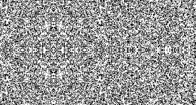
Now that we have a nice framework for running the simulation, we can start finding interesting rules. The naive way to do this is to just create random rule strings. This can create interesting results, but usually it just produces boring noise-like rules:

How about just modifying game of life? Well what we can do is just flip a single bit of a rule’s bitstring. Unfortunately, since Game of Life is very unusual rule in our set, adjacent rules aren’t actually very interesting.

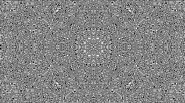
Instead, let’s start with a cool maze generator rule I found randomly (there are a lot of rules like this):

Flip a single bit, and we get:

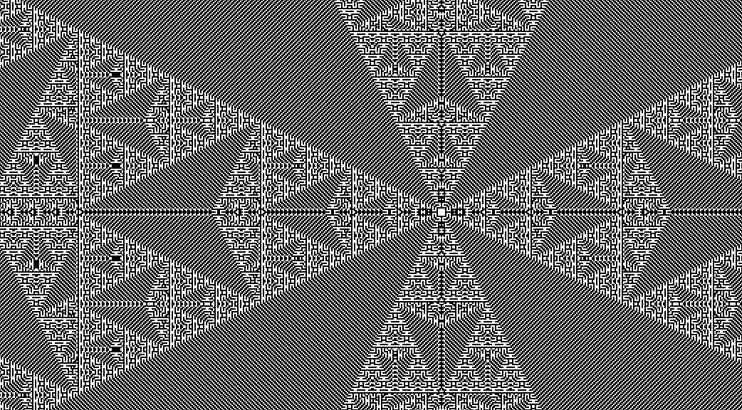
Sierpinski arrowheads! Very different and interesting, and only a single bit away. Let’s do it again:

By iterating existing rules in this way, we can often produce fun new rules. I have already found almost a dozen rules by this process, which I have included as presets in the simulator. Check it out and try and find some yourself!

Next Steps#

Well now we have a functioning cellular automata simular running in the browser. It’s extremely fast because it runs on the GPU, as well as very dynamic, as arbitrary rules can be passed as textures to the fragment shader.

Next, we’ll look at expanding our set of possible rules by allowing more than two possible states. It will be a little complicated, as the way we specify rules will have to change. Not only will there be multiple possible input states (remember our rule is really a function), but also multiple quantities of neighbors. If we have 4 neighbors of state A, we can only have a maximum total of 4 for other states B, C, D, etc. If we want our rule texture to occupy the least possible space, we need to think carefuly about representation.

This will allow us to simulate some really interesting rules like Brian’s Brain (3 states), Wireworld (4 states), Codd’s CA (8 states), and any other totalistic rule we can think of! At some point, we’ll also take a look at non-totalistic rules, which will allow an absolutely astounding rule space (more possible rules than particles in the universe!)

Stay tuned!